从 GeometricField 到 fvMatrix

GeometricField 和 fvMatrix 是 OpenFOAM 中的两个重要的类。本文将试图分析这两个类的源码实现及其用法。

GeometricField 类

GeometricField 是用来描述几何场信息的类模板（class template）。注意这是一个模板（template），而不是类（class）。因此需要将 GeometricField 实例化（instantiation）形成具体的类才能使用。

模板参数

GeometricField 有三个模板参数：Type、PatchField 和 GeoMesh。其声明如下：

1
2
3
4
5
6

template<class Type, template<class> class PatchField, class GeoMesh>
class GeometricField
:
    public DimensionedField<Type, GeoMesh>
{
    // ...

模板参数的含义如下：

注意：其中的 PatchField 也是一个类模板，Type 是它的模板参数，在 GeometricField 类的代码中以 PatchField<Type> 形式出现，实例化以后的类型为 fvPatchField<scalar> 或 fvsPatchField<vector> 等。

为了简写，实例化之后的 GeometricField 都有别名，如 volScalarField，volVectorField、surfaceScalarField 等。这些别名在以下文件中定义：

• src/finiteVolume/fields/volFields/volFieldsFwd.H
• src/finiteVolume/fields/surfaceFields/surfaceFieldsFwd.H

继承关系

GeometricField 继承自 DimensionedField， 而 DimensionedField 继承自 regIOobject 和 Field，Field 又继承自 refCount 和 List。因此 GeometricField 具有以上所有类的属性和功能。

GeometricField 的继承关系

• List 是一个列表，可以认为它是一个特殊的数组。

• refCount 是实现引用计数功能的类，派生自它的所有类都有一个引用计数器。在执行拷贝时并不会真正的将数据在内存中复制一份，而仅仅将引用计数器加一。

• Field 是一个用来描述场的类，继承自 refCount 和 List，因此具有以上两者的属性和功能。

• regIOobject 是用于实现注册对象输出输出的类，派生自 regIOobject 的子类可以利用 OpenFOAM 的注册对象机制实现自动读取和写入文件的功能。

主要成员变量

GeometricField 的主要成员变量如下：

• timeIndex_:当前时间步索引

• field0Ptr_: 指向上一时间步场量的指针

• fieldPrevIterPtr_: 指向上一迭代步场量的指针（用于亚松驰）

• boundaryField_: 边界上的场量

可见，与 DimensionedField 相比，它多了与时间步进、数值迭代相关的一些成员变量。

此外，为了方便简写，它还定义了几个类型别名：

 1
 2
 3
 4
 5
 6
 7
 8
 9
10
11
12
13

        //- Type of mesh on which this GeometricField is instantiated
        typedef typename GeoMesh::Mesh Mesh;

        //- Type of boundary mesh on which this
        //  GeometricField::Boundary is instantiated
        typedef typename GeoMesh::BoundaryMesh BoundaryMesh;

        //- Type of the internal field from which this GeometricField is derived
        typedef DimensionedField<Type, GeoMesh> Internal;

        //- Type of the patch field of which the
        //  GeometricField::Boundary is composed
        typedef PatchField<Type> Patch;

举例来说，若实例化的类型为 volScalarField，那么这些别名对应的实际类型如下：

• Mesh $\rightarrow$ fvMesh

• BoundaryMesh $\rightarrow$ fvMesh::BoundaryMesh $\rightarrow$ fvMesh::fvBoundaryMesh

• Internal $\rightarrow$ DimensionedField<scalar, volMesh>

• Patch $\rightarrow$ PatchField<scalar> $\rightarrow$ fvPatchField<scalar>

主要成员函数

• storeOldTimes(): 更新 field0Ptr_ 的值。先判断当前场量是否以 _0 结尾，若不满足条件则调用 storeOldTime()。
• storeOldTime(): 更新 field0Ptr_ 的值。被 storeOldTimes() 调用。
• storePrevIter(): 更新 fieldPrevIter_ 的值。
• correctBoundaryConditions(): 执行 boundaryField_.evaluate() ，更新边界上的值。
• needReference(): 判断是否需要参考值。如果有边界为 fixed-value 或 mixed （Robin边界条件） ，则返回 false，否则返回 true。
• relax(): 从字典文件中相关参数，决定是否对场量进行亚松驰。

 1
 2
 3
 4
 5
 6
 7
 8
 9
10
11
12
13
14
15
16
17
18
19
20
21
22
23
24

template<class Type, template<class> class PatchField, class GeoMesh>
void Foam::GeometricField<Type, PatchField, GeoMesh>::relax()
{
    word name = this->name();

    if
    (
        this->mesh().data::template lookupOrDefault<bool>
        (
            "finalIteration",
            false
        )
    )
    {
        name += "Final";
    }

    // 若 fvSolution.relaxationFactors.fields.name 存在则返回 true
    if (this->mesh().relaxField(name))
    {
        // 用 fvSolution.relaxationFactors.fields.name 对应的因子对场量进行松弛
        relax(this->mesh().fieldRelaxationFactor(name));
    }
}

默认的场量松弛因子为 0，即不松驰。

用法

GeometricField 本身是一个数组，它的索引按照 GeoMesh 不同而不同。对于 volMesh，以网格单元编号为索引。对于 surfaceMesh，以面单元编号为索引 。

GeometricField 的定义有以下几种情形：

• 从文件读取。通常在算例初始化的时候定义，将场量（如速度、压力等）从文件中读取到内存中。代码位于求解器中的 createFields.H 文件。如：

 1
 2
 3
 4
 5
 6
 7
 8
 9
10
11
12

     volVectorField U
     (
         IOobject
         (
             "U",
             runTime.timeName(),
             mesh,
             IOobject::MUST_READ,
             IOobject::AUTO_WRITE
         ),
         mesh
     );

这种情况是用 IOobject 和 fvMesh 构建一个 GeometricField 对象。它会读取 U 文件中的 internalField 和 boundaryField 的对应值到内存中。

• 从函数返回。如：

1

    tmp<volTensorField> tgradU = fvc::grad(U);

fvc::grad(U) 返回的是一个 tmp 封装的 volTensorField 类型，直接赋值即可。

• 从其他场量计算得到。这种情况一般不用 GeometricField ，而用 GeometricField::Internal（即 DimensionedField）定义（见 OpenFOAM-dev@a25a449 和 OpenFOAM-dev@02dd851）。

fvMatrix 类

fvMatrix 是用来表示离散矩阵的一个类模板。注意它也是模板，而不是类，也需要进行实例化后才能使用。

模板参数

fvMatrix 只有一个模板参数Type，它表示用来离散的物理量的类型，如 scalar，vector 等。其声明如下：

1
2
3
4
5
6
7

template<class Type>
class fvMatrix
:
    public tmp<fvMatrix<Type>>::refCount,
    public lduMatrix
{
    // ...

继承关系

在旧版本（4.0 以前）的代码中，fvMatrix 继承自 refCount，4.0 及以后的版本继承自一个用 tmp 封装类中的 refCount 类（见 OpenFOAM-dev@cd59748）。此外，fvMatrix 还是 lduMatrix 的子类。lduMatrix 是将有限体积的网格关系剥离后形成的一个类，它用于存储稀疏矩阵。下面会介绍它具体是如何存储的。

主要成员变量

• psi_: 用来离散的场量的引用。
• dimensions_: 量纲。
• source_: 源项，不计入边界条件影响。
• internalCoeffs_: 边界条件对系数矩阵 A 的影响。
• boundaryCoeffs_: 边界条件对源项 b 的影响。
• faceFluxCorrectionPtr_: 非正交网格修正中的面通量。

主要成员函数

• setReference: 设置参考值。修改参考单元对应的对角元素和源项，来修改目标网格单元的值。
• relax(const scalar alpha): 对方程进行亚松驰。主要对对角元素和源项进行亚松驰。
• boundaryManipulate(): 实现边界条件对矩阵系数修改的操作。调用 bFields[patchi].manipulateMatrix(*this) 达到修改矩阵系数的目的。
• D(): 返回主对角元素，计入边界条件影响。
• A(): 返回 D() 除以网格体积（注意是 volScalarField）。
• H(): 返回 H 运算的结果。

用法

先介绍系数矩阵是如何存储的。lduMatrix 将矩阵分为三部分存储，分别是对角元素、上三角元素和下三角元素。以上三部分是不考虑边界条件影响的离散系数矩阵，分别用 lduMatrix<Type>::diag()、lduMatrix<Type>::upper() 和 lduMatrix<Type>::lower() 访问。

1. 若网格单元数为 $N$，则离散后的矩阵是一个 $N \times N$ 的稀疏矩阵。
2. 矩阵的行和列编号对应网格单元编号。
3. 第 $i$ 行的主对角元素 $A_{ii}$ 对应第 $i$ 个网格的系数。
4. 第 $i$ 行的非零对角元素 $A_{ij}$ 反应的是第 $j$ 个网格对第 $i$ 个网格的影响。
5. 非零对角元素的位置由第 $i$ 个网格的相邻网格的编号确定。
6. 相邻网格的编号通过面单元寻址，每个面单元都有一个 owner 和一个 neighbour。
7. 遍历面单元。若面单元的 owner 编号为 $i$，则其 neighbour 对应的编号为非零元素。若面单元的 neighbour编号为 $i$，则其 owner 对应的编号为非零元素。
8. 由于 OpenFOAM 采用 owner < neighbour 的网格编号原则，因此上条的第一种情况非零元素为上三角元素，第二种情况非零元素为下三角元素。

三个函数的具体原理如下：

• diag() 按顺序返回所有的主对角元素。
• upper() 返回的是上三角元素，通过 upperAddr() 寻址， upperAddr() 在 fvMeshLduAddressing 中定义，返回的是mesh.faceNeighbour()，即面单元的 neighbour。
• lower() 返回的是下三角元素，通过 loweraddr() 寻址，lowerAddr() 也在 fvMeshLduAddressing 中定义，返回的是 mesh.faceOwner() 的一个子列表（面单元包括边界上的面单元，这些单元只有 owner，没有 neighbour，因此 owner 会比 neighbour 多）。

注意这里只是单纯的离散系数矩阵，还未将边界条件的影响考虑进来。边界套件的影响放在 internalCoeffs_ 和 boundaryCoeffs_ 中，在需要的时候通过 addCmptAvBoundaryDiag 、addBoundaryDiag 和 addBoundarySource 等函数施加。

从 GeometricField 到 fvMatrix

GeometricField 是用来描述网格上的物理量信息的类，而 fvMatrix 是用来描述离散后的稀疏线性方程组系统的类。从 GeometricField 到 fvMatrix 的过程即为将物理场变成稀疏线性方程组的离散过程。

fvMatrix 的构造函数并未对系数矩阵和源项做任何操作，因此定义 fvMatrix 对象的时候系数矩阵和源项是空的。对其进行赋值的操作在 fvm:: 命名空间中的各个函数中进行，如 fvm::div，fvm::laplacian 等。

为了形象地说明整个离散过程，我们选用 Versteeg 写的 An Introduction to Computational Fluid Dynamics: The Finite Volume Method (2nd Edition) 一书中的两个例子来演示。

一维扩散问题

Example 4.1

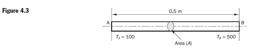
Consider the problem of source-free heat conduction in an insulated rod whose ends are maintained at constant temperatures of 100°C and 500°C respectively. The one-dimensional problem sketched in Figure 4.3 is governed by

$$ \frac{d}{dx}\left( k \frac{dT}{dx}\right) = 0 $$

Calculate the steady state temperature distribution in the rod. Thermal conductivity $k$ equals 1000 $\mathrm{W/m\cdot K}$, cross-sectional area $A$ is $10 \times 10^{−3} \mathrm{m}^2$.

选用 laplacianFoam 作为求解器来演示，选用 closedVolume 算例进行修改。步骤如下：

• 将 closedVolume 拷贝至 $FOAM_RUN 并改名为 1ddiffusion

1
2

cp -r $FOAM_ETC/templates/closedVolume $FOAM_RUN/1ddiffusion
cd $FOAM_RUN/1ddiffusion

• 修改 system/blockMeshDict 中的计算域大小

 1
 2
 3
 4
 5
 6
 7
 8
 9
10
11
12

backgroundMesh
{
    xMin     0;
    xMax     0.5;
    yMin     0;
    yMax     0.1;
    zMin     0;
    zMax     0.1;
    xCells   5;
    yCells   1;
    zCells   1;
}

• 修改 system/blockMeshDict 中的边界名（未命名的剩余边界都叫 defaultFaces）

 1
 2
 3
 4
 5
 6
 7
 8
 9
10
11
12
13
14
15
16
17
18
19
20

boundary
{
    inlet
    {
        type patch;
        faces
        (
            (0 4 7 3)
        );
    }

    outlet
    {
        type patch;
        faces
        (
            (1 5 6 2)
        );
    }
}

• 修改 0/T 中的边界条件（defaultFaces 默认为 empty，此处可省略）

 1
 2
 3
 4
 5
 6
 7
 8
 9
10
11
12
13
14

boundaryField
{
    inlet
    {
        type            fixedValue;
        value           uniform 100;
    }

    outlet
    {
        type            fixedValue;
        value           uniform 500;
    }
}

• 修改 constant/transportProperties 中的导热率

1

DT              DT [0 2 -1 0 0 0 0] 1000;

• 修改 constant/turbulenceProperties，关掉湍流模拟

1

simulationType laminar;

• 执行 blockMesh 划分网格

这样算例便准备完了。接下来需要对求解器进行修改，输出我们需要的信息

• 拷贝求解器源码

1

cp -r $FOAM_APP/solvers/basic/laplacianFoam .

• 修改编译输出目录和输出文件名

1
2
3

cd laplacianFoam
sed -i 's/FOAM_APPBIN/FOAM_USER_APPBIN/' Make/files
sed -i 's/laplacianFoam$/myLaplacianFoam/' Make/files

• 修改求解器源码 laplacianFoam.C，在 fvOptions.constrain(TEqn); 上方加上以下输出语句

1
2
3
4
5
6
7
8
9

    Info<< "diag(): " << TEqn.diag() << endl;
    Info<< "upper(): " << TEqn.upper() << endl;
    Info<< "lower(): " << TEqn.lower() << endl;
    Info<< "source(): " << TEqn.source() << endl;
    Info<< "upperAddr(): " << TEqn.lduAddr().upperAddr() << endl;
    Info<< "lowerAddr(): " << TEqn.lduAddr().lowerAddr() << endl;
    Info<< "internalCoeffs():" << TEqn.internalCoeffs() << endl;
    Info<< "boundaryCoeffs():" << TEqn.boundaryCoeffs() << endl;
    Info<< "D(): " << TEqn.D() << endl;

• 执行 wmake 编译新的求解器

• 到算例目录执行 myLaplacianFoam，求解器输出如下：

diag(): 5(100 200 200 200 100)
upper(): 4(-100 -100 -100 -100)
lower(): 4(-100 -100 -100 -100)
source(): 5(0 0 8.8817995e-13 -8.8817995e-13 0)
upperAddr(): 4(1 2 3 4)
lowerAddr(): 4(0 1 2 3)
internalCoeffs():
3
(
1(200)
1(200)
0()
)

boundaryCoeffs():
3
(
1(20000)
1(100000)
0()
)

D(): 5(300 200 200 200 300)

整个组装后的矩阵方程如下：

$$ \left[ \begin{array}{ccccc} \color{red}{100}\color{black}{+}\color{magenta}{200} & \color{green}{-100} & 0 & 0 & 0 \newline \color{blue}{-100} & \color{red}{200} & \color{green}{-100} & 0 & 0 \newline 0 & \color{blue}{-100} & \color{red}{200} & \color{green}{-100} & 0 \newline 0 & 0 & \color{blue}{-100} & \color{red}{200} & \color{green}{-100} \newline 0 & 0 & 0 & \color{blue}{-100} & \color{red}{100}\color{black}{+}\color{magenta}{200} \newline \end{array} \right] \left[ \begin{array}{c} T_1 \newline T_2 \newline T_3 \newline T_4 \newline T_5 \newline \end{array} \right] = \left[ \begin{array}{c} \color{aqua}{0} \color{black}{+} \color{olive}{20000} \newline \color{aqua}{0} \newline \color{aqua}{0} \newline \color{aqua}{0} \newline \color{aqua}{0} \color{black}{+} \color{olive}{100000} \newline \end{array} \right] $$

其中,

• 红色部分为 diag()
• 绿色部分为 upper()
• 蓝色部分为 lower()
• 海蓝色部分为 source()
• 洋红色部分为 internalCoeffs()
• 橄榄色部分为 boundaryCoeffs()

那么 internalCoeffs 和 boundaryCoeffs 是如何施加到矩阵上的呢？ 这两个均为 FieldField 类型，可以看成是一个数组封装另一个数组。外层数组的长度为边界数量，上面的例子中有三个边界（inlet，outlet和defaultFaces），所以长度为 3。内层数组为边界条件施加到系数和源项上的值，对应的单元通过 fvLduAddressing 中的 patchAddr 函数寻址得到。

在求解器中增加输出 patchAddr 的源码，如下：

1
2
3
4

    forAll(mesh.boundary(), patchi)
    {
        Info<< "patchAddr for " << mesh.boundary()[patchi].name() << ": " << TEqn.lduAddr().patchAddr(patchi) << endl;
    }

重新编译求解器并运行，输出如下：

patchAddr for inlet: 1(0)
patchAddr for outlet: 1(4)
patchAddr for defaultFaces: 0()

说明 inlet 的影响施加在第 1 个网格单元，outlet 的影响施加在第 5 个网格单元，defaultFaces 不影响系数矩阵。

一维对流扩散问题

Example 5.1

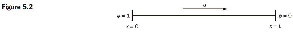
A property $\phi$ is transported by means of convection and diffusion through the one-dimensional domain sketched in Figure 5.2. The governing equation is

$$ \frac{d}{dx}(\rho u \phi) = \frac{d}{dx}\left(\Gamma \frac{d\phi}{dx}\right) $$

The boundary conditions are $\phi_0 = 1$ at $x = 0$ and $\phi_L = 0$ at $x = L$. Using five equally spaced cells and the central differencing scheme for convection and diffusion, calculate the distribution of $\phi$ as a function of $x$ for (i) Case 1: $u$ = 0.1 m/s, (ii) …

The following data apply: length $L = 1.0$ m, $\rho = 1.0 \mathrm{kg/m}^3$, $\Gamma = 0.1 \mathrm{kg/m \cdot s}$.

选用 scalarTransportFoam 作为求解器来演示，同样选用 closedVolume 算例进行修改。由于密度为1，为了方便说明，在离散的时候将密度省去。

• 将 closedVolume 拷贝至 $FOAM_RUN 并改名为 1dconvectiondiffusion

1
2

cp -r $FOAM_ETC/templates/closedVolume $FOAM_RUN/1dconvectiondiffusion
cd $FOAM_RUN/1dconvectiondiffusion

• 修改 system/blockMeshDict 中的计算域大小

 1
 2
 3
 4
 5
 6
 7
 8
 9
10
11
12

backgroundMesh
{
    xMin     0;
    xMax     1;
    yMin     0;
    yMax     1;
    zMin     0;
    zMax     1;
    xCells   5;
    yCells   1;
    zCells   1;
}

• 修改 system/blockMeshDict 中的边界名（未命名的剩余边界都叫 defaultFaces）

 1
 2
 3
 4
 5
 6
 7
 8
 9
10
11
12
13
14
15
16
17
18
19
20

boundary
{
    inlet
    {
        type patch;
        faces
        (
            (0 4 7 3)
        );
    }

    outlet
    {
        type patch;
        faces
        (
            (1 5 6 2)
        );
    }
}

• 修改 0/T 中的边界条件（defaultFaces 默认为 empty，此处可省略）

 1
 2
 3
 4
 5
 6
 7
 8
 9
10
11
12
13
14

boundaryField
{
    inlet
    {
        type            fixedValue;
        value           uniform 1;
    }

    outlet
    {
        type            fixedValue;
        value           uniform 0;
    }
}

• 修改 0/U 中的初始条件和边界条件（defaultFaces 默认为 empty，此处可省略）

 1
 2
 3
 4
 5
 6
 7
 8
 9
10
11
12
13
14
15
16

internalField   uniform (0.1 0 0);

boundaryField
{
    inlet
    {
        type            fixedValue;
        value           uniform (0.1 0 0);
    }

    outlet
    {
        type            fixedValue;
        value           uniform (0.1 0 0);
    }
}

• 修改 constant/transportProperties 中的扩散系数

1

DT              DT [0 2 -1 0 0 0 0] 0.1;

• 修改 constant/turbulenceProperties，关掉湍流模拟

1

simulationType laminar;

• 执行 blockMesh 划分网格

这样算例便准备完了。接下来需要对求解器进行修改，输出我们需要的信息

• 拷贝求解器源码

1

cp -r $FOAM_APP/solvers/basic/scalarTransportFoam .

• 修改编译输出目录和输出文件名

1
2
3

cd scalarTransportFoam
sed -i 's/FOAM_APPBIN/FOAM_USER_APPBIN/' Make/files
sed -i 's/scalarTransportFoam$/myScalarTransportFoam/' Make/files

• 修改求解器源码 scalarTransportFoam.C，在 TEqn.relax(); 上方加上以下输出语句

1
2
3
4
5
6
7
8
9

    Info<< "diag(): " << TEqn.diag() << endl;
    Info<< "upper(): " << TEqn.upper() << endl;
    Info<< "lower(): " << TEqn.lower() << endl;
    Info<< "source(): " << TEqn.source() << endl;
    Info<< "upperAddr(): " << TEqn.lduAddr().upperAddr() << endl;
    Info<< "lowerAddr(): " << TEqn.lduAddr().lowerAddr() << endl;
    Info<< "internalCoeffs():" << TEqn.internalCoeffs() << endl;
    Info<< "boundaryCoeffs():" << TEqn.boundaryCoeffs() << endl;
    Info<< "D(): " << TEqn.D() << endl;

• 执行 wmake 编译新的求解器

• 到算例目录执行 myScalarTransportFoam，求解器输出如下：

diag(): 5(0.55 1 1 1 0.45)
upper(): 4(-0.45 -0.45 -0.45 -0.45)
lower(): 4(-0.55 -0.55 -0.55 -0.55)
source(): 5(0 0 -1.1856535e-17 1.1856535e-17 0)
upperAddr(): 4(1 2 3 4)
lowerAddr(): 4(0 1 2 3)
internalCoeffs():
3
(
1(1)
1(1)
0()
)

boundaryCoeffs():
3
(
1(1.1)
1(0)
0()
)

D(): 5(1.55 1 1 1 1.45)

整个组装后的矩阵方程如下： $$ \left[ \begin{array}{ccccc} \color{red}{0.55}\color{black}{+}\color{magenta}1 & \color{green}{-0.45} & 0 & 0 & 0 \newline \color{blue}{-0.55} & \color{red}{1} & \color{green}{-0.45} & 0 & 0 \newline 0 & \color{blue}{-0.55} & \color{red}{1} & \color{green}{-0.45} & 0 \newline 0 & 0 & \color{blue}{-0.55} & \color{red}{1} & \color{green}{-0.45} \newline 0 & 0 & 0 & \color{blue}{-0.55} & \color{red}{0.45}\color{black}{+}\color{magenta}{1} \newline \end{array} \right] \left[ \begin{array}{c} \phi_1 \newline \phi_2 \newline \phi_3 \newline \phi_4 \newline \phi_5 \newline \end{array} \right] = \left[ \begin{array}{c} \color{aqua}{0} \color{black}{+} \color{olive}{1.1} \newline \color{aqua}{0} \newline \color{aqua}{0} \newline \color{aqua}{0} \newline \color{aqua}{0} \color{black}{+} \color{olive}{0} \newline \end{array} \right] $$ 加入对流项后，最终的形成矩阵是非对称的。

将对流项和扩散项拆分开来，对求解器进行修改，增加以下代码：

 1
 2
 3
 4
 5
 6
 7
 8
 9
10
11
12
13
14
15
16
17
18
19

    fvScalarMatrix TEqnConvection(fvm::div(phi, T));
    Info<< "Convection term diag(): " << TEqnConvection.diag() << endl;
    Info<< "Convection term upper(): " << TEqnConvection.upper() << endl;
    Info<< "Convection term lower(): " << TEqnConvection.lower() << endl;
    Info<< "Convection term source(): " << TEqnConvection.source() << endl;
    Info<< "Convection term internalCoeffs():" << TEqnConvection.internalCoeffs() << endl;
    Info<< "Convection term boundaryCoeffs():" << TEqnConvection.boundaryCoeffs() << endl;
    Info<< "Convection term D(): " << TEqnConvection.D() << endl;

    Info<< endl;

    fvScalarMatrix TEqnDiffusion(-fvm::laplacian(DT, T));
    Info<< "Diffusion term diag(): " << TEqnDiffusion.diag() << endl;
    Info<< "Diffusion term upper(): " << TEqnDiffusion.upper() << endl;
    Info<< "Diffusion term lower(): " << TEqnDiffusion.lower() << endl;
    Info<< "Diffusion term source(): " << TEqnDiffusion.source() << endl;
    Info<< "Diffusion term internalCoeffs():" << TEqnDiffusion.internalCoeffs() << endl;
    Info<< "Diffusion term boundaryCoeffs():" << TEqnDiffusion.boundaryCoeffs() << endl;
    Info<< "Diffusion term D(): " << TEqnDiffusion.D() << endl;

求解器输出如下：

D(): 5(1.55 1 1 1 1.45)
Convection term diag(): 5(0.05 1.3877788e-17 3.469447e-17 -4.8572257e-17 -0.05)
Convection term upper(): 4(0.05 0.05 0.05 0.05)
Convection term lower(): 4(-0.05 -0.05 -0.05 -0.05)
Convection term source(): 5{0}
Convection term internalCoeffs():
3
(
1(-0)
1(0)
0()
)

Convection term boundaryCoeffs():
3
(
1(0.1)
1(-0)
0()
)

Convection term D(): 5(0.05 1.3877788e-17 3.469447e-17 -4.8572257e-17 -0.05)

Diffusion term diag(): 5(0.5 1 1 1 0.5)
Diffusion term upper(): 4(-0.5 -0.5 -0.5 -0.5)
Diffusion term lower(): 4(-0.5 -0.5 -0.5 -0.5)
Diffusion term source(): 5(-0 -0 -1.1856535e-17 1.1856535e-17 -0)
Diffusion term internalCoeffs():
3
(
1(1)
1(1)
0()
)

Diffusion term boundaryCoeffs():
3
(
1(1)
1(0)
0()
)

Diffusion term D(): 5(1.5 1 1 1 1.5)

对流项的离散系数方程

$$ \left[ \begin{array}{ccccc} \color{red}{0.05} & \color{green}{0.05} & 0 & 0 & 0 \newline \color{blue}{-0.05} & \color{red}{0} & \color{green}{0.05} & 0 & 0 \newline 0 & \color{blue}{-0.05} & \color{red}{0} & \color{green}{0.05} & 0 \newline 0 & 0 & \color{blue}{-0.05} & \color{red}{0} & \color{green}{0.05} \newline 0 & 0 & 0 & \color{blue}{-0.05} & \color{red}{-0.05} \newline \end{array} \right] \left[ \begin{array}{c} \phi_1 \newline \phi_2 \newline \phi_3 \newline \phi_4 \newline \phi_5 \newline \end{array} \right] = \left[ \begin{array}{c} \color{aqua}{0} \color{black}{+} \color{olive}{0.1} \newline \color{aqua}{0} \newline \color{aqua}{0} \newline \color{aqua}{0} \newline \color{aqua}{0} \color{black}{+} \color{olive}{0} \newline \end{array} \right] $$

扩散项的离散系数方程

$$ \left[ \begin{array}{ccccc} \color{red}{0.5}\color{black}{+}\color{magenta}1 & \color{green}{-0.5} & 0 & 0 & 0 \newline \color{blue}{-0.5} & \color{red}{1} & \color{green}{-0.5} & 0 & 0 \newline 0 & \color{blue}{-0.5} & \color{red}{1} & \color{green}{-0.5} & 0 \newline 0 & 0 & \color{blue}{-0.5} & \color{red}{1} & \color{green}{-0.5} \newline 0 & 0 & 0 & \color{blue}{-0.5} & \color{red}{0.5}\color{black}{+}\color{magenta}{1} \newline \end{array} \right] \left[ \begin{array}{c} \phi_1 \newline \phi_2 \newline \phi_3 \newline \phi_4 \newline \phi_5 \newline \end{array} \right] = \left[ \begin{array}{c} \color{aqua}{0} \color{black}{+} \color{olive}{1} \newline \color{aqua}{0} \newline \color{aqua}{0} \newline \color{aqua}{0} \newline \color{aqua}{0} \color{black}{+} \color{olive}{0} \newline \end{array} \right] $$

将方程对应的矩阵和源项相加即得到了之前组装的矩阵方程。

（完）